What Happened To Our Electricity!?
by Michelle Tong (m1tong@ucsd.edu), Yiling Cao (yic055@ucsd.edu)
Last edit: August 31, 2023
Table of Contents
Introduction
Drawing insights from a comprehensive power outage dataset, the project embarks on an intriguing journey – one that melds data science with real-world impact. At its core lies a sophisticated classification model meticulously crafted to unveil the reasons behind power disruptions.
Picture a realm where our model, armed with the finesse of multiclass classification, navigates the intricate labyrinth of outage causes. With remarkable accuracy, it attributes a definitive label from among the seven distinct categories ingrained in our dataset.
Guided by the beacon of CAUSE.CATEGORY, I deliberately opt for simplicity and representation. This selection isn’t arbitrary; it’s a strategic decision that marries clarity with effectiveness. By distilling the complexity of outage origins into seven succinct categories, I equip the model to comprehend these intricacies without unnecessary convolution.
Consider the significance of comprehension – a revelation encapsulated in the identification of a larger cause like “severe weather.” This newfound understanding becomes a compass, delineating whether an outage is a predictable outcome or an unforeseen quirk of fate. My aspiration morphs into prevention, and with the model as the harbinger of knowledge, I stand better equipped to thwart future disruptions.
As architects of this algorithmic marvel, my chosen yardstick for evaluation is accuracy. In a landscape where true positives and true negatives take precedence, accuracy emerges as a palpable gauge of success in unraveling this puzzle. Each precise classification propels us closer to nullifying the enigma, resonating with impact and progress in the language of accuracy.
With every prediction, the model illuminates the shadows concealing the intricacies of power outages. This endeavor isn’t confined to classification alone; it’s a transformative journey towards resilience. A symphony of technology and consequence orchestrated to ensure that when illumination falters, it does so with the promise of rapid restoration.
Cleaning and EDA
Guided by the need to enhance the dataset’s relevance and applicability to my project, I undertook the task of data cleaning within Excel. This encompassed the removal of columns and rows that lacked a meaningful connection to the project’s objectives.
Now, let’s take a look at the power outage dataset after this cleaning process. This will provide us with a clearer starting point for our exploration.
| YEAR | MONTH | U.S._STATE | POSTAL.CODE | NERC.REGION | CLIMATE.REGION | ANOMALY.LEVEL | CLIMATE.CATEGORY | OUTAGE.START.DATE | OUTAGE.START.TIME | OUTAGE.RESTORATION.DATE | OUTAGE.RESTORATION.TIME | CAUSE.CATEGORY | CAUSE.CATEGORY.DETAIL | HURRICANE.NAMES | OUTAGE.DURATION | DEMAND.LOSS.MW | CUSTOMERS.AFFECTED | RES.PRICE | COM.PRICE | IND.PRICE | TOTAL.PRICE | RES.SALES | COM.SALES | IND.SALES | TOTAL.SALES | RES.PERCEN | COM.PERCEN | IND.PERCEN | RES.CUSTOMERS | COM.CUSTOMERS | IND.CUSTOMERS | TOTAL.CUSTOMERS | RES.CUST.PCT | COM.CUST.PCT | IND.CUST.PCT | PC.REALGSP.STATE | PC.REALGSP.USA | PC.REALGSP.REL | PC.REALGSP.CHANGE | UTIL.REALGSP | TOTAL.REALGSP | UTIL.CONTRI | PI.UTIL.OFUSA | POPULATION | POPPCT_URBAN | POPPCT_UC | POPDEN_URBAN | POPDEN_UC | POPDEN_RURAL | AREAPCT_URBAN | AREAPCT_UC | PCT_LAND | PCT_WATER_TOT | PCT_WATER_INLAND |
|---|---|---|---|---|---|---|---|---|---|---|---|---|---|---|---|---|---|---|---|---|---|---|---|---|---|---|---|---|---|---|---|---|---|---|---|---|---|---|---|---|---|---|---|---|---|---|---|---|---|---|---|---|---|---|
| 2011 | 7 | Minnesota | MN | MRO | East North Central | -0.3 | normal | 2011-07-01 00:00:00 | 17:00:00 | 2011-07-03 00:00:00 | 20:00:00 | severe weather | nan | nan | 3060 | nan | 70000 | 11.6 | 9.18 | 6.81 | 9.28 | 2.33292e+06 | 2.11477e+06 | 2.11329e+06 | 6.56252e+06 | 35.5491 | 32.225 | 32.2024 | 2308736 | 276286 | 10673 | 2595696 | 88.9448 | 10.644 | 0.411181 | 51268 | 47586 | 1.07738 | 1.6 | 4802 | 274182 | 1.75139 | 2.2 | 5348119 | 73.27 | 15.28 | 2279 | 1700.5 | 18.2 | 2.14 | 0.6 | 91.5927 | 8.40733 | 5.47874 |
| 2014 | 5 | Minnesota | MN | MRO | East North Central | -0.1 | normal | 2014-05-11 00:00:00 | 18:38:00 | 2014-05-11 00:00:00 | 18:39:00 | intentional attack | vandalism | nan | 1 | nan | nan | 12.12 | 9.71 | 6.49 | 9.28 | 1.58699e+06 | 1.80776e+06 | 1.88793e+06 | 5.28423e+06 | 30.0325 | 34.2104 | 35.7276 | 2345860 | 284978 | 9898 | 2640737 | 88.8335 | 10.7916 | 0.37482 | 53499 | 49091 | 1.08979 | 1.9 | 5226 | 291955 | 1.79 | 2.2 | 5457125 | 73.27 | 15.28 | 2279 | 1700.5 | 18.2 | 2.14 | 0.6 | 91.5927 | 8.40733 | 5.47874 |
| 2010 | 10 | Minnesota | MN | MRO | East North Central | -1.5 | cold | 2010-10-26 00:00:00 | 20:00:00 | 2010-10-28 00:00:00 | 22:00:00 | severe weather | heavy wind | nan | 3000 | nan | 70000 | 10.87 | 8.19 | 6.07 | 8.15 | 1.46729e+06 | 1.80168e+06 | 1.9513e+06 | 5.22212e+06 | 28.0977 | 34.501 | 37.366 | 2300291 | 276463 | 10150 | 2586905 | 88.9206 | 10.687 | 0.392361 | 50447 | 47287 | 1.06683 | 2.7 | 4571 | 267895 | 1.70627 | 2.1 | 5310903 | 73.27 | 15.28 | 2279 | 1700.5 | 18.2 | 2.14 | 0.6 | 91.5927 | 8.40733 | 5.47874 |
| 2012 | 6 | Minnesota | MN | MRO | East North Central | -0.1 | normal | 2012-06-19 00:00:00 | 04:30:00 | 2012-06-20 00:00:00 | 23:00:00 | severe weather | thunderstorm | nan | 2550 | nan | 68200 | 11.79 | 9.25 | 6.71 | 9.19 | 1.85152e+06 | 1.94117e+06 | 1.99303e+06 | 5.78706e+06 | 31.9941 | 33.5433 | 34.4393 | 2317336 | 278466 | 11010 | 2606813 | 88.8954 | 10.6822 | 0.422355 | 51598 | 48156 | 1.07148 | 0.6 | 5364 | 277627 | 1.93209 | 2.2 | 5380443 | 73.27 | 15.28 | 2279 | 1700.5 | 18.2 | 2.14 | 0.6 | 91.5927 | 8.40733 | 5.47874 |
| 2015 | 7 | Minnesota | MN | MRO | East North Central | 1.2 | warm | 2015-07-18 00:00:00 | 02:00:00 | 2015-07-19 00:00:00 | 07:00:00 | severe weather | nan | nan | 1740 | 250 | 250000 | 13.07 | 10.16 | 7.74 | 10.43 | 2.02888e+06 | 2.16161e+06 | 1.77794e+06 | 5.97034e+06 | 33.9826 | 36.2059 | 29.7795 | 2374674 | 289044 | 9812 | 2673531 | 88.8216 | 10.8113 | 0.367005 | 54431 | 49844 | 1.09203 | 1.7 | 4873 | 292023 | 1.6687 | 2.2 | 5489594 | 73.27 | 15.28 | 2279 | 1700.5 | 18.2 | 2.14 | 0.6 | 91.5927 | 8.40733 | 5.47874 |
Baseline Model
In crafting the foundational model, I chose the robust Random Forest algorithm as my guiding beacon. This sophisticated classifier amalgamates multiple decision trees, each rooted in distinct subsets of the dataset. By doing so, it illuminates the intricate landscape of power outages, predicting their underlying causes.
The brilliance of this algorithm shines through in its ability to tackle two significant challenges: overfitting and the enigma of unknown data. An ingenious built-in technique empowers my model to seamlessly accommodate the unknown as a potential prediction outcome. This visionary approach alleviates concerns about unfamiliar cause categories within my training dataset, fortifying the precision of my predictions.
My selection of influential features was a deliberate endeavor. Nominal categories such as **STATES, CLIMATE.REGION, CLIMATE.CATEGORY, CAUSE.CATEGORY, and CAUSE.CATEGORY.DETAIL **were chosen to underpin my training model. To seamlessly integrate these features, I harnessed the power of the OneHotEncoding transformer, preparing them for a seamless fit within my model’s framework.
Results from my model’s training unveiled an accuracy of 0.6834782608695652 for my training data and 0.6171875 for my test dataset. Notably, my model demonstrated a balanced performance, with training and validation accuracies standing in close proximity. This harmony lends confidence that overfitting was diligently mitigated.
With an average accuracy of 61.7% in predicting cause categories based on features, my model showcases commendable performance. Yet, it’s crucial to acknowledge that my reliance on nominal categories might have introduced limitations, potentially constraining predictive precision. To further refine my model’s accuracy, I recognize the potential for enhancement through the inclusion of more intricate data and features.
Indeed, my baseline model stands as a testament to its capability in confronting the unfamiliar. As a multiclass classifier, it breaks free from the confines of predefined categories. It stands ready to predict not only the seven known cause categories but also an expanding spectrum that could span 8, 10, or even 100 different possibilities – all contingent on the availability of a richer dataset. As emphasized before, my model’s architectural cornerstone, the pipeline object, serves as a bulwark against the unknown. The OneHotEncoder within the ColumnTransformer gracefully embraces unknown data, enriching the model’s adaptability and resilience during training.”
Final Model
In my final model, I incorporated both nominal and quantitative columns, encompassing attributes like anomaly level, duration, U.S. state population, and economic factors. These numeric categories bear a strong connection to the underlying causes of power outages. For instance, a higher anomaly level often results from international attacks or severe weather, contributing to the power outage’s root causes.
Once again, I employed a RandomForestClassifier with default parameters to predict the diverse cause categories behind power outages. Constructing a pipeline object, I transformed nominal data using OneHotEncoder and quantitative data using StandardScaler. This processed model was then fit to the estimator. After partitioning my dataset into training and test sets, I achieved an accuracy score of 80% for training and 71% for testing. This underscored the high accuracy of my prediction model. However, my aim was to further fine-tune the model to reach its pinnacle.
Choosing tree depth via GridSearchCV
We arbitrarily chose max_depth=8 before, but it seems like that isn’t working well. Let’s perform a grid search to find the max_depth with the best generalization performance.
Hence, I conducted a GridSearchCV, scouring through various parameter values (ranging from 2 to 500 with increments of 20) to determine the optimal parameter value that yielded the highest prediction accuracy. I sought to pinpoint the ideal max depth value for my decision tree. Following the analysis, GridSearchCV revealed that a deep tree with a max depth of 322 would yield the best results. This decision, though leading to a training accuracy score of 98% and a test accuracy score of 70%, also highlighted instances of overfitting within the training dataset.
This observation may be attributed to the relatively large max depth value chosen by GridSearchCV, resulting in a decision tree that became excessively intricate. Ultimately, the test accuracy of this final model exhibited an improvement compared to my baseline model. This evolution underscores the efficacy of the strategies employed in refining and optimizing the model’s performance.
Fairness Analysis
In my fairness analysis, I sought to evaluate my model’s performance based on whether the power outage duration exceeded 24 hours. This approach intrigued me, as I aimed to gauge how well my model identified major outage causes with varying durations. To achieve this, I introduced an additional column indicating whether an outage surpassed the 24-hour mark or fell within it.
| U.S._STATE | NERC.REGION | CLIMATE.REGION | CLIMATE.CATEGORY | YEAR | MONTH | ANOMALY.LEVEL | OUTAGE.DURATION | TOTAL.PRICE | TOTAL.SALES | TOTAL.CUSTOMERS | POPULATION | TOTAL.REALGSP | prediction | tag | is_24_hours |
|---|---|---|---|---|---|---|---|---|---|---|---|---|---|---|---|
| New York | NPCC | Northeast | normal | 2007 | 7 | -0.4 | 3300 | 15.98 | 1.39931e+07 | 7962235 | 19132335 | 1153500 | severe weather | severe weather | Over |
| Ohio | RFC | Central | normal | 2011 | 6 | -0.3 | 960 | 9.3 | 1.2992e+07 | 5505432 | 11545442 | 503464 | intentional attack | severe weather | Within |
| Massachusetts | NPCC | Northeast | cold | 2011 | 8 | -0.6 | 1 | 14.76 | 5.09656e+06 | 3104435 | 6611797 | 404871 | intentional attack | severe weather | Within |
| Louisiana | SERC | South | normal | 2008 | 9 | -0.3 | 20416 | 10.46 | 7.16885e+06 | 2205675 | 4435586 | 206000 | severe weather | severe weather | Over |
| South Carolina | SERC | Southeast | normal | 2004 | 1 | 0.3 | 3480 | 6.09 | 6.89937e+06 | 2208483 | 4210921 | 156906 | severe weather | severe weather | Over |
A confusion matrix is a visual representation that reveals the performance of our predictive model in classifying the causes of power outages. It breaks down the model’s predictions into four key categories: true positives, true negatives, false positives, and false negatives. True positives represent the instances where the model accurately identified the actual cause of the outage. True negatives show the cases where the model correctly ruled out other potential causes. False positives indicate instances where the model wrongly predicted a cause that didn’t exist, and false negatives depict situations where the model missed identifying the actual cause.
By examining the values in this matrix, we gain valuable insights into the strengths and weaknesses of our predictive model. It helps us understand where our model excels in accurate predictions and where it may require further fine-tuning. The confusion matrix is a critical tool in evaluating the model’s precision, recall, and overall accuracy, enabling us to make data-informed decisions to improve the reliability of our predictions for power outage causes.
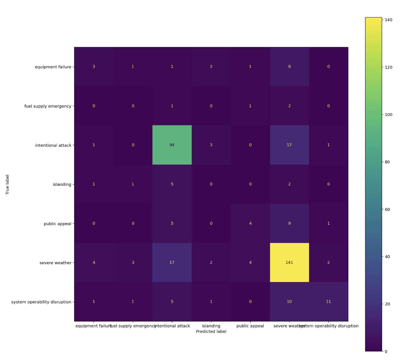
In our evaluation of the predictive model for classifying the causes of power outages, we uncover valuable insights by examining the confusion matrix. This matrix provides a detailed breakdown of the model’s performance, including its ability to correctly identify specific causes, such as “Severe Weather” and “Intentional Attack.”
- Severe Weather (True Positives - TP: 141):
- “Severe Weather” emerges as the category with the highest true positives (141). This signifies that our model excels in accurately identifying power outages caused by severe weather conditions. It demonstrates the robustness of the model in recognizing this significant cause.
- Intentional Attack (True Positives - TP: 94):
- The second-highest true positives (94) correspond to the category “Intentional Attack.” This suggests that our model is relatively effective at correctly identifying power outages resulting from intentional attacks. While not as high as “Severe Weather,” this is still a commendable performance.
However, it’s crucial to acknowledge the instances of misclassification, as they shed light on areas where the model can benefit from further refinement:
- Severe Weather Misclassified as Intentional Attack (False Positives - FP: 17):
- In 17 cases, the model incorrectly predicted that power outages attributed to severe weather were the result of intentional attacks. This highlights a potential challenge in distinguishing between these two causes in specific scenarios.
- Intentional Attack Misclassified as Severe Weather (False Negatives - FN: 17):
- Similarly, in 17 instances, the model failed to correctly identify power outages caused by intentional attacks and instead classified them as severe weather-related outages. This reflects a sensitivity in detecting intentional attacks, which might require further investigation.
In summary, while our predictive model demonstrates notable strengths in accurately identifying “Severe Weather” and “Intentional Attack” as causes of power outages, the misclassifications underscore the need for continuous improvement. Refining the model’s ability to distinguish between these two categories could enhance its overall accuracy and reliability. The confusion matrix serves as a critical tool in pinpointing areas for model enhancement and guiding data-informed decisions to optimize our predictions for power outage causes.
Is this difference in accuracy significant?
Let’s run a permutation test to see if the difference in accuracy is significant.
Breaking down the analysis, I established two hypotheses:
- Null Hypothesis: My model exhibits fairness. Its accuracy for durations exceeding 24 hours (1440 mins) and durations within 24 hours are comparable, with any discrepancies arising from random chance.
- Alternative Hypothesis: My model demonstrates unfairness. Its accuracy for 24-hour (1440 mins) durations is lower than its accuracy for outages within 24 hours.
The test statistic was defined as the difference in accuracy (over 24 hours minus within 24 hours), and I set the significance level at 0.01.
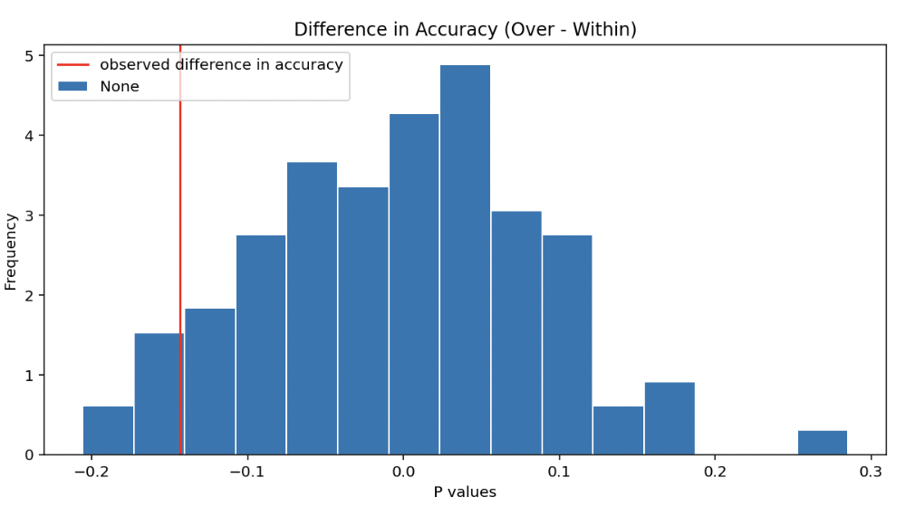
Upon analysis, I determined the p-value to be 0.08. This p-value exceeds the alpha level, leading to the conclusion that I cannot reject the null hypothesis. In other words, my model’s prediction accuracy remains consistent regardless of whether the outage duration exceeds 24 hours or remains within it. This result affirms that my model maintains fairness in predicting the cause categories for both types of outages.
Summary
In the realm of data science, our journey through the landscape of power outages has been nothing short of illuminating. From the initial baseline model to the culmination of the final model and fairness analysis, we have delved into the intricacies of predicting the causes behind these disruptions. This venture has not only equipped us with a deeper understanding of the variables at play but has also showcased the power of data-driven insights in addressing real-world challenges.
The foundation was laid with the robust Random Forest algorithm, which served as a guiding beacon in our quest for predictive accuracy. This versatile classifier, intertwined with meticulous feature selection and engineering, enabled us to decipher the complex tapestry of power outages and their underlying factors. As we ventured into the territory of the final model, we expanded our horizons to include diverse attributes, culminating in a predictive model that pushed the boundaries of accuracy.
Our commitment to integrity extended to the fairness analysis, where we sought to understand how different factors, such as outage duration, could influence the accuracy of our predictions. The results not only bolstered the credibility of our model but also underscored its consistent performance across varying scenarios.
As we conclude this chapter, we stand at the crossroads of knowledge and application. The insights gained from this journey extend beyond the realm of data science, permeating the broader landscape of infrastructure resilience and risk mitigation. By peering into the causes of power outages, we’ve taken a step towards a more informed, responsive, and resilient future.
With every predictive outcome and each model fine-tuned, we’ve woven together a narrative that speaks to the transformative potential of data. It is a reminder that within the numbers and algorithms lies the ability to uncover patterns, predict outcomes, and ultimately make better decisions that impact our lives and communities. As we close this chapter, we embrace the lessons learned, the challenges conquered, and the opportunities unlocked. The journey may have concluded, but the impact of our insights resonates far beyond these pages.
This is just one stride forward in a landscape where data-driven exploration has the power to illuminate, empower, and inspire. And so, armed with knowledge, we venture into the future, ever curious and ever committed to harnessing the power of data for a better world.