Congestion Prediction in IC Design using Graph Neural Network
Uses different Graph Neural Networks (GNNs) to predict congestion in IC design to accelerate optimization processes and address challenges in layout complexities.
Introducion
Predicting congestion in IC design is a critical yet challenging task. Congestion occurs when excessive wiring or routing is required in certain regions of the chip layout, often resulting from suboptimal floor planning or high cell density. This can lead to significant issues, such as timing discrepancies, crosstalk, increased power consumption, reduced reliability, and high production costs. Early prediction and mitigation of congestion are thus essential to avoid these complications.
Current optimization tools for calculating congestion are extremely time-consuming given the complexity of modern chips. A machine learning model that utilizes the existing information of netlists and their congestion can accelerate the optimization process in IC design. Predicting congestion is generally complex due to the intricate nature of IC layouts. This project seeks to address this challenge by leveraging Graph Neural Networks (GNNs), which hold promise due to their ability to model complex relationships and interactions in graph-structured data.
Related Work: The approach of using graph neural networks in congestion prediction has been explored in recent works. Kirby et al. utilized deep Graph Attention Networks on the hypergraph representation of IC designs to predict congestion
Given the advantages of GNNs in circuit congestion prediction, our project aims to explore similar GNN architectures from Kirby et al.’s work on the NCSU-DigIC-GraphData dataset and compare the performance of different GNN architectures. NCSU-DigIC-GraphData has a much smaller scale compared to the netlists used in Kirby et al.’s paper, which has roughly 50 million cells from tens of designs. Experimenting with graph neural networks on different sizes of netlists can give us insights into how well GNNs scale and how different GNN architectures perform on a smaller-scale dataset.
Methodology
Dataset
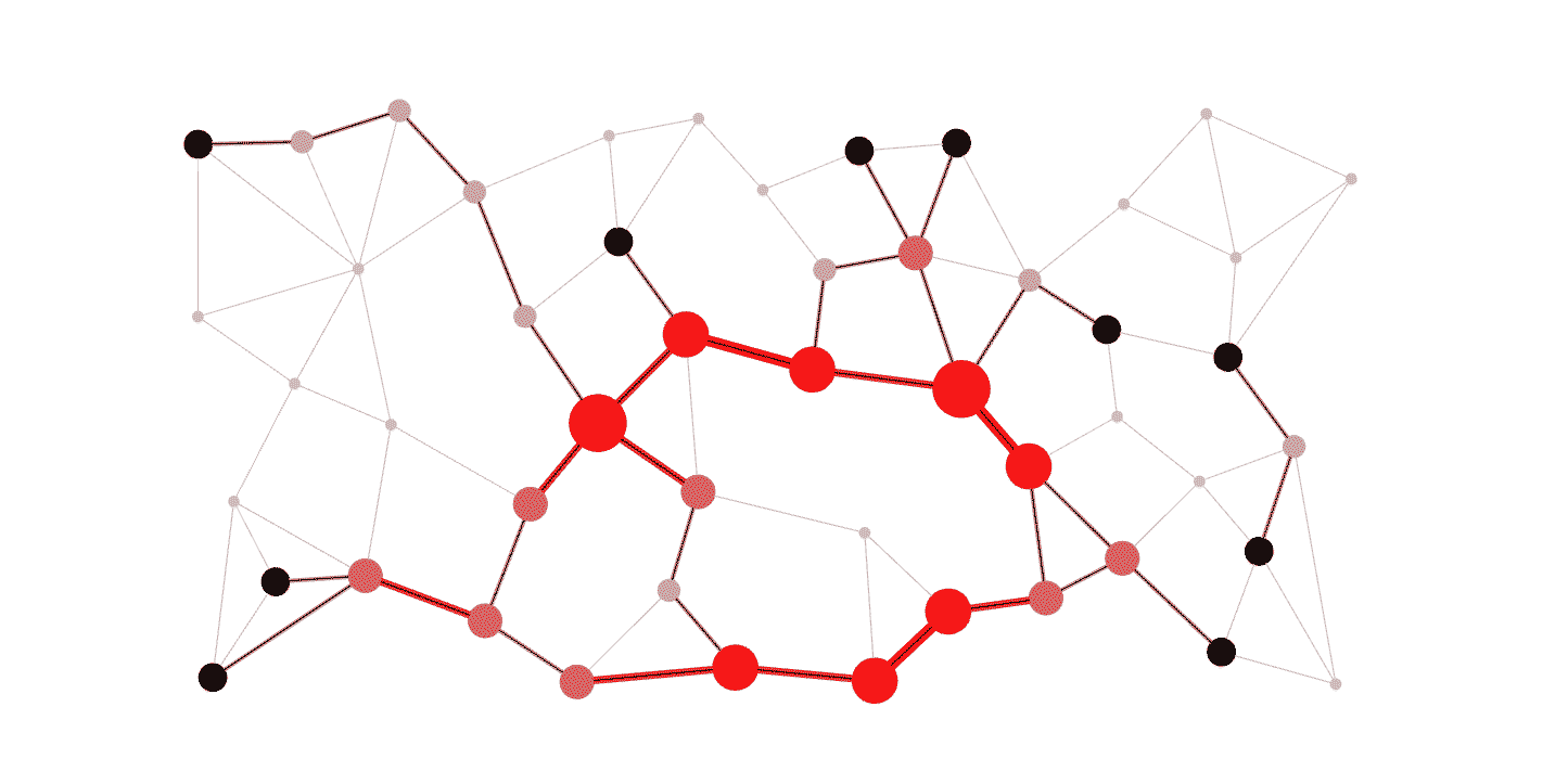
This project utilizes the NCSU-DigIC-GraphData, which comprises 13 netlists, each exhibiting unique placement and congestion characteristics. For each netlist, the dataset contains node features, node connectivity, and Global Route Cell (GRC) based demand and capacity. GRCs are organized in a rectangular grid (Figure 1), but not all GRCs have the same dimensions.
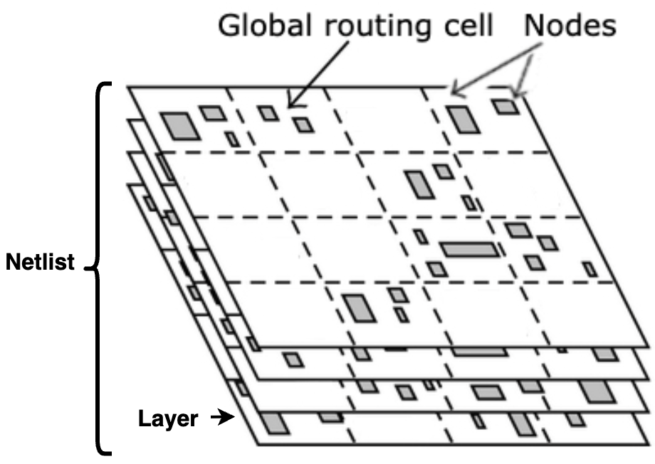
Figure 1a
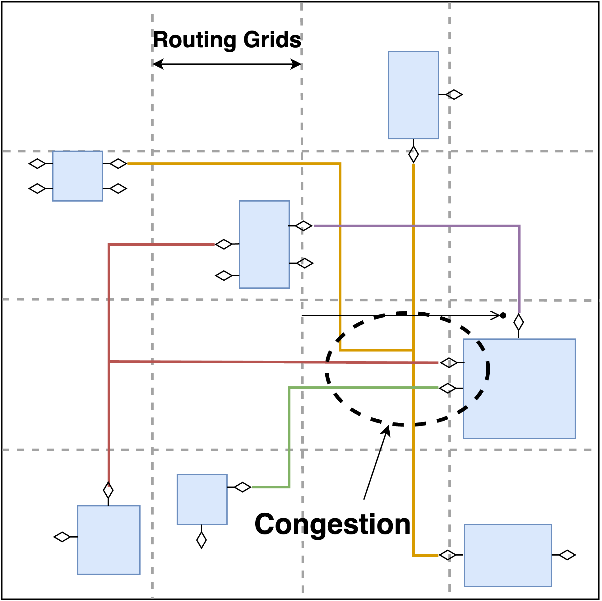
Figure 1b
For each netlist, the dataset contains node features, node connectivity, and GRC based congestion (demand minus capacity). Node features and node connectivity refer to the characteristics and interconnections of individual elements within the netlist. GRC-based congestion calculates congestion at a GRC index with multiple nodes.
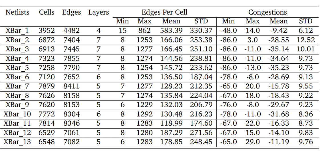
Table 1: Dataset'details & statistics. 1st column in the table shows the name of each netlist, 2nd-4th column show the number of cells, edge, and effective layers in each netlist, 5th-8th columns show the distribution of edge per cells for each netlist and 9th-12th columns show the distribution of congestions for each netlist.
Feature Selection and Engineering
Selecting node features is essential for training the Graph Neural Network (GNN). The dataset gives basic node features, including the locations of nodes, the dimensions of the cells, and their orientations, as detailed below:
-
xloc and yloc: The locations of nodes (xloc and yloc) provide the relative positions for the model to learn where congestion typically occurs within the chip layout.
-
width and height: Utilizing the size of the nodes, specifically the width and height of the cells, serves as a convenient method to encode the cell type directly into the model, offering insights into the physical space occupied by each element.
-
orient: The orientation of the cells might indicate the preferred direction of routing, offering a hint towards potential congestion areas.
Besides the existing node features, some related features are calculated and assigned to each node.
-
cell density: The number of cells inside each GRC. By assigning cell densities to nodes, the model can use them to reference how congested different areas are.
-
input and output degrees: The number of connections a node has to other nodes. It serves as critical routing information and helps with the prediction task.
-
GRC Indexes: Unique x and y index for each GRC. Even though xloc and yloc already encode the spatial information of nodes, GRC indexes can provide extra references for the model to understand the spatial relationships of nodes.
To examine the correlation between these features and demand/congestion. We calculated the Pearson correlation coefficients (Table 2). In the table, we removed height and orientation because all cells have the same height and orientation is not ordinal. The correlation coefficients indicate an association between selected features and targeted congestion.
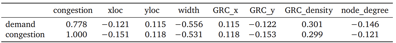
Table 2: Correlation Table
As one can observe, the correlation between congestion and demand is very high (0.778). As stated before, congestion is defined as (demand - capacity). In other words, the existence of demand is what causes congestion, which explains why the correlation between these two variables is notably high. Therefore, we will consider the idea of constructing a model that predicts demand instead of congestion.
To ensure our model’s robustness across various designs, feature normalization is performed. The xloc, yloc, width, and height values are normalized before being fed into the model, allowing it to generalize across designs with differing dimensions. The orientation feature (orient) is encoded using one-hot encoding to capture its categorical nature effectively.
Additionally, connectivity data is transformed into an Edge Index using the adjacency matrix, an important step for enabling the GNN to understand the connections between nodes. This Edge Index serves as a key input, allowing the network to learn the intricate relationships and pathways within the graph structure.
Congestion/Demand data, combined from all layers, is mapped to each node based on the Global Route Cell (GRC) boundaries. Congestion can be computed as the difference between demand and capacity, providing a quantitative measure of congestion at each node.
Graph Neural Network
Our project employs Graph Convolutional Network (GCN) and Graph Attention Network (GAT) architectures.
GCN Model
GCN models utilize the graph-based structure of circuit designs, where nodes represent circuit components, and edges denote connections between these components. The model utilizes spatial dependencies between components to predict congestion by encoding both local and global structures of the circuit.
Architecture Details:
-
Node Feature Encoding: Each node $v_i$ in the circuit graph $G(V,E)$ is associated with a feature vector $x_i$ that represents the physical properties of the circuit components, such as size, orientation, and connectivity.
-
Graph Convolution Layers: The model comprises multiple graph convolution layers. Each layer transforms the node features into higher-level representations. A graph convolution layer is defined as:
\[H^{(l+1)} = \sigma(\tilde{D}^{-\frac{1}{2}} \tilde{A} \tilde{D}^{-\frac{1}{2}} H^{(l)} W^{(l)})\]where $H^{(l)}$ is the matrix of node features at layer $l$, $\tilde{A} = A + I$ is the adjacency matrix $A$ with added self-loops $I$, $\tilde{D}$ is the degree matrix of $\tilde{A}$, $W^{(l)}$ is the weight matrix for layer $l$, and $\sigma$ denotes a nonlinear activation function such as ReLU. This equation is given by Kipf et al. [1].
-
Pooling and Readout: After several graph convolution layers, a global pooling layer aggregates the node features to capture the overall graph structure. The readout layer maps these aggregated features to congestion predictions.
GAT Model
To refine the model’s capability in capturing intricate dependencies between circuit components, we incorporate a Graph Attention Network (GAT) layer, which assigns varying importance to different nodes within a neighborhood. The equations below are derived from Veličković et al.
Architecture Details:
-
Attention Mechanism: The GAT layer computes attention coefficients for node pairs, indicating the importance of node $j$’s features to node $i$:
\[\alpha_{ij} = \frac{\exp(\text{LeakyReLU}(\mathbf{a}^\top[W h_i \| W h_j]))}{\sum_{k \in N_i} \exp(\text{LeakyReLU}(\mathbf{a}^\top[W h_i \| W h_k]))}\]where $h_i$ and $h_j$ are the feature vectors of nodes $i$ and $j$, respectively, $W$ is a shared weight matrix, $\mathbf{a}$ is the attention mechanism’s weight vector, and $N_i$ denotes the neighbors of node $i$.
-
Multi-head Attention: To stabilize the learning process, we employ multi-head attention, where $K$ independent attention mechanisms execute in parallel, and their features are concatenated. This leads to the following representation for each node:
\[\text{MultiHead}(h_i) = \big\|_{k=1}^K \sigma \left( \sum_{j \in N_i} \alpha_{ij}^k W^k h_j \right)\]where $\big|_{k=1}^K$ denotes concatenation of the outputs from $K$ attention heads.
-
Integration into GCN: The GAT layers are integrated with the GCN framework, allowing the model to leverage both the structured feature propagation of GCNs and the adaptive attention mechanism of GATs for enhanced congestion prediction.
GRC-Based Prediction Model
Since the demand and capacity data is stored per GRC, predicting congestion per GRC may have better performance compared to predicting congestion per node. Furthermore, per node prediction fails to predict congestion for GRCs that are empty. Therefore, we decide to test a GRC-based model architecture alongside with node-based model.
To utilize GNNs, we treat each GRC as a node and compute GRC features and GRC edge index. GRC features are the averages of node features in each GRC. Empty GRCs are imputed using their neighbors’ features. GRC edge index is derived from the node edge index. Duplicate edges are retained to preserve the connectivity information between GRCs.
Results
Node-Based Models
By training the GCN model on one netlist (Xbar_1) that contains 3952 nodes, it reached a training loss of 75.368 and a test loss of 82.583. From Figure 2a, we can tell that the training and validation loss decreased exponentially and are healthy.
When we plotted the scatterplots of ground truth demand and predicted demand (Figure 2b), we found that our model tends to predict the mean of the congestion. This may be due to the MSE loss function we used. It reflects that the model failed to capture the relationship between node features, connectivity, and demand.
On the other hand, the GAT model reached a training loss of 15.083 and a test loss of 13.418 (Figure 2c&d). Moreover, Pearson’s correlation coefficient for the predicted demand and ground truth is 0.472 for the GAT model, much higher than the correlation coefficient of the GCN model (0.005). To test our models’ robustness, we separately trained the GCN and GAT models on every design and calculated the RMSE, Pearson’s r, Kendell’s Tau B on the test sets.

Figure 2a
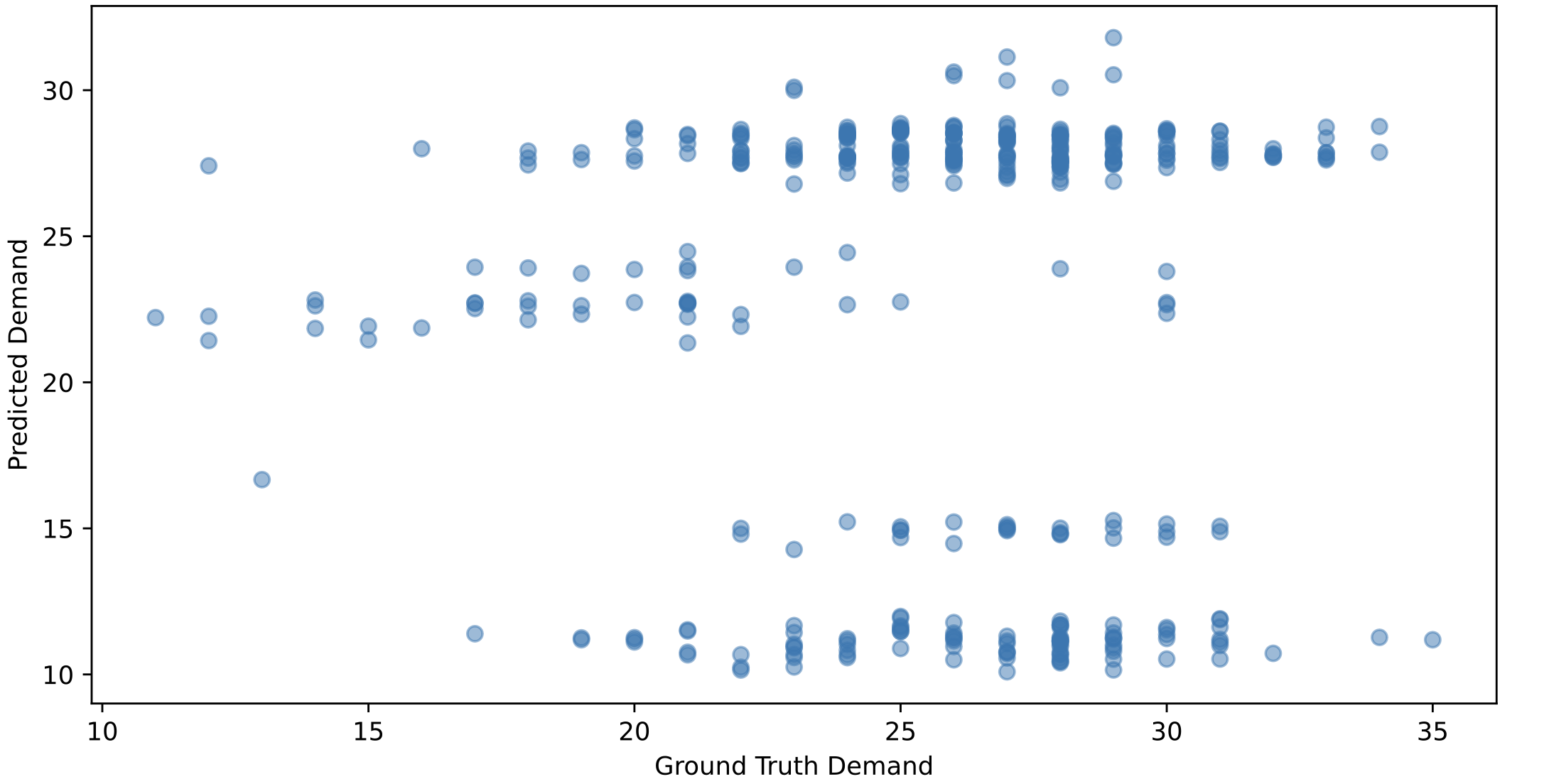
Figure 2b
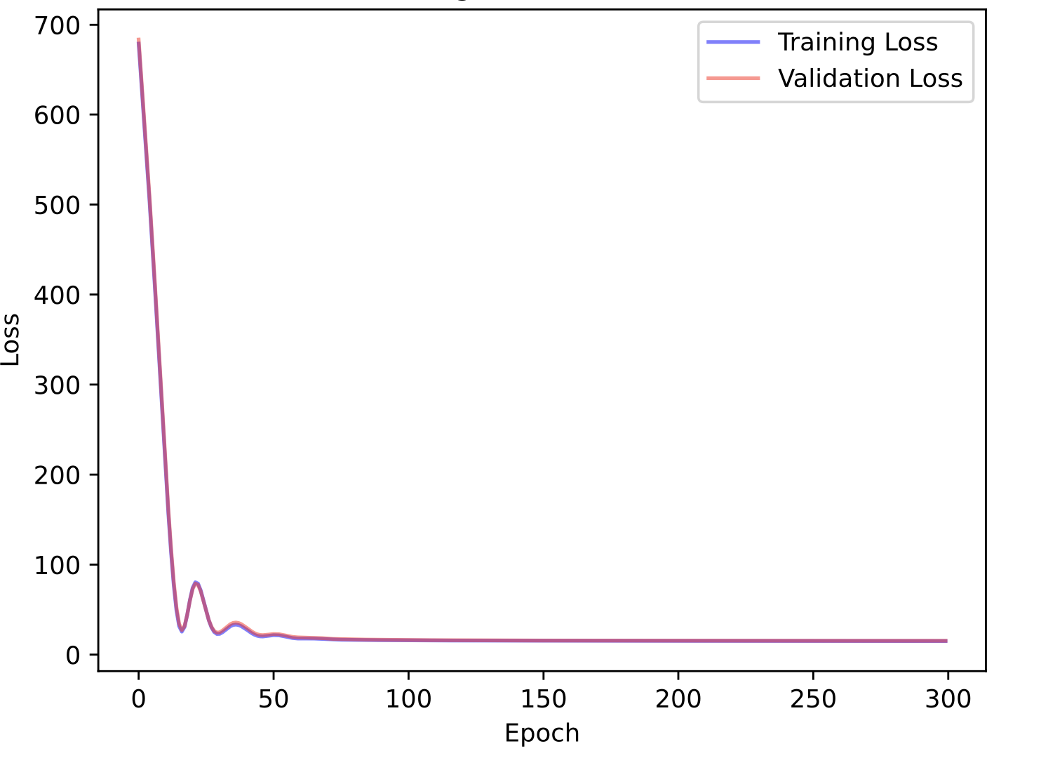
Figure 2c

Figure 2d
Table 3 contains model performance on single designs and cross designs settings. The performance of a naive mean predictor is also included to serve as a reference for model performance. Generally, GATs have lower RMSE and higher Pearson and Kendall in both single-design training and cross-design training compared to GCNs.
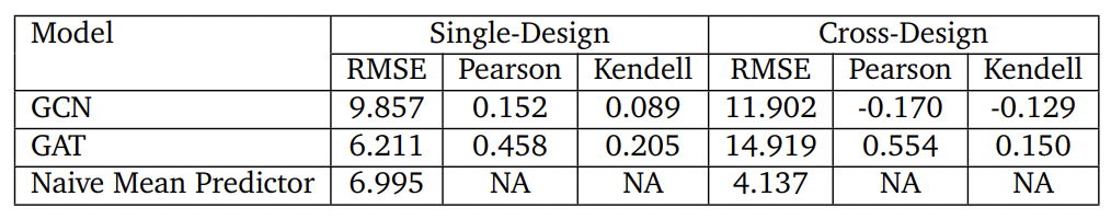
Table 3: Model Performance Comparison
GRC-Based Models
We experimented with a per GRC prediction model using a GAT model because we believed GRC-based models may have the lowest MSE given the nature of how demand is stored in the dataset. However, the prediction has the worst correlation coefficient with the ground truth (-0.0855) compared to cell-based models. Figure 3 shows the prediction has no patterns at all. This might be caused by a lack of node features in the GRC-based models.
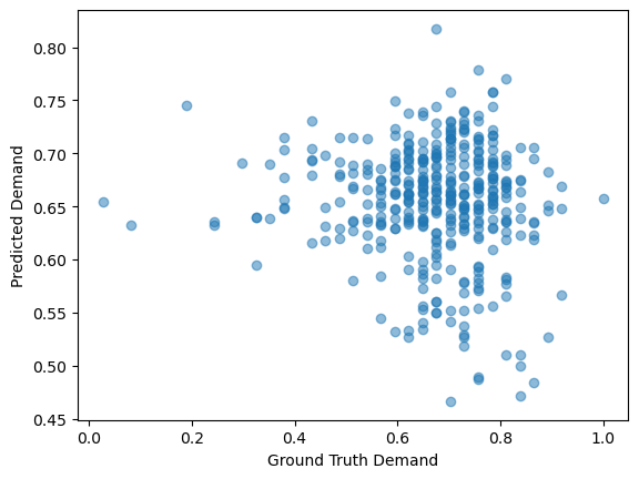
Figure 3
Conclusion
In this project, we have tested both GCN and GAT models on the NCSU-DigIC-GraphData dataset. We discovered that models trained on one netlist are not robust and tend to vary a lot in terms of MSE and Correlation Coefficient. We compared GAT’s performance on a single design and multiple designs and observed better results than GCN models. However, we noticed that GAT can take more time to train compared to GCN models if we increase the number of heads in the attention mechanisms. Node-based models are superior to GRC-based models based on their performance and robustness. Overall, GCN models perform worse than a naive mean predictor, while GAT models are slightly better than a naive mean predictor, indicting the poor scalability of GNN models on small netlists.